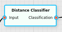
Distance Classifier Filter

Classifies individual pixels based on their distance to reference training data.

Category	Classification
Node
Parameters	MatchMethod: whether to match against the averages of the reference training data (Centroid) or to match against each individual data point (pixel) of the reference training data (KNN) DistanceMethod: how to calculate the distance: Cosine for a scalar product (akin to a spectral angle mapper, SAM); Euclidean for a simple distance norm; Mahalanobis for a Mahalanobis distance norm; and CIEDE2000 for the $\Delta E$ distance as specified in the CIE 2000 standard (requires Lab* color values as input) Classification Threshold: the threshold that excludes a match from being considered KNN: the number of closest individual points to consider when MatchMethod is KNN BaseQuantity: whether the threshold and optional output should be in the raw distance (Distances) or an abstract similarity level (Similarity Level) Maximum Results: the maximum number of matches to output Output Configuration/Base Quantity: whether the distances or similarity levels for each classification result should be output in a second output of this filter Applicable (group specific): whether a specific group should be considered for this filter
Inputs	Input/Color: the input data to classify
Outputs	Classification: the classification result Similarity Level/Distance (optional): the similarity level and/or distance for each classification result

Effect of the Filter

The filter requires input data where individual data points (pixels) were assigned to various groups. This classifier learns this labelled data and during execution compares them to the input data it receives. It will then assign to each data point (pixel) a class (or “unclassified” if there was no match) that the input resembles most closely.

Only groups that have been marked Applicable in the parameters are considered for this filter. (By default all groups are considered applicable.)

Background

The filter automatically takes into account all pixels that were assigned to be background (if any). If the background is closer to any given input data than any group, the pixel will be considered unclassified, regardless of whether a group still has some similarity.

Number of results

The filter can return more than a single classification result per pixel; if the Maximum Results parameter is set to a value larger than one, the classification result will contain all groups that match the data, sorted by how good they fit the data.

For example, if a user defines groups G1, G2, and G3, and a pixel is similar enough to groups G1 and G3 that the threshold still lets them through, the pixel will be classified as G1 and G3, with the order being chosen so that the best match comes first.

Note

There is a jump in processing time when switching from one result being returned to two or more results being returned.

Cetroid vs. KNN

The filter can be applied in two different modes: in the default mode, where the MatchMethod parameter is set to Centroid, the labelled input data points will be averaged for each group. During execution each new data point will be compared to the average of each group, and the matches will be ordered by the best match, until cut off by the threshold.

In KNN mode all of the individual labelled data points will be remembered by the filter, and during execution each new data point will be compared to the k closest training data points, where k is the value of the KNN parameter. The group with the most data points in that set that match the data being processed will be considered the closest match. In case of a tie the group with the closest distance will win.

Warning

The KNN mode will be quite slow, especially if the number of training data points is large.

This only describes how the

Cosine (Spectral Angle Mapper, SAM)

If DistanceMethod is set to Cosine the distance between the input spectra and the training spectra will be calculated via the formula:

$d = 1 - \left| \frac{\mathbf{y} \cdot \mathbf{y}_{\mathrm{ref}}}{\left\Vert\mathbf{y}\right\Vert \left\Vert\mathbf{y}_{\mathrm{ref}}\right\Vert} \right|$

The distance range will vary between 0 and 1. This mode is best used when applying this filter directly to data with many channels, such as spectra. It is often not very useful when applied to data with only a handful of channels, and in the limit where the number of channels is 1 the distance will always be 0, regardless of the input.

This manner of classifying spectra is sometimes also referred to as spectral angle mapper, or SAM, because the scalar product calculates the cosine of the angle between the vectors in an abstract space.

Euclidean Distance

If DistanceMethod is Euclidean this will calculate the simple Euclidean distance between the input data and the training data, assuming they live in an abstract vector space. It will use the formula

$d = \left| \mathbf{y} - \mathbf{y}_{\mathrm{ref}} \right|_2$

This is most useful when applying the distance classifier to data where the dimensionality of the input data has already been reduced to a few channels. It is not recommended to use this when applying it to pure spectral reflectance data.

Common methods of dimensionality reduction include the Principal Component Analysis and the Linear Discriminant Analysis.

Mahalanobis Distance

If DistanceMethod is Mahalanobis it will calculate a distance similar to the Euclidean case, but it will consider the shape of the distribution of the training data when it comes to calculating the distances. It will use the expression

$d = \sqrt{(\mathbf{y} - \mathbf{y}_{\mathrm{ref}})^{\mathrm{T}} C^{-1} (\mathbf{y} - \mathbf{y}_{\mathrm{ref}})}$

where $C^{-1}$ is the inverse covariance matrix for the given reference group for $\mathbf{y}_{\mathrm{ref}}$ . The following diagram illustrates this:

_images/distanceclassifier_mahalanobis.svg

Here we see two distributions of training data, A and B, and a point P. In the Euclidean case the point P has a very similar distance to both groups. In the Mahalanobis case the point P will be considered closer to group B, because of how the group lies in the abstract space.

CIE DeltaE 2000 Distance

If DistanceMethod is set to CIEDE2000 then the input must consist of color values in the CIE L*a*b* color space. The classifier will then calculate the distance based on the standardized formula for calculating $\Delta E$ according to the CIE 2000 standard.

Base Quantity (Similarity Level vs. Distance)

The Base Quantity parameter will dictate how the Classification Threshold parameter and the optional second output of the filter will be interpreted.

If Base Quantity is set to Distance then the threshold will be given in the distance as described in the previous sections. Any distance to training data that is larger than the threshold will cause the classifier to assume that the given group does not match the input data. The optional second output will output the distances corresponding to each successful classification result, or positive infinity if no groups could be found that were closer than the specified threshold.

If Base Quantity is set to Similarity Level then the distances will be converted into a similarty level that ranges from 0 (not similar at all) to 1 (identical). The threshold must be provided in that range from 0 to 1; any similarity level that is smaller than the threshold will cause the classifier to assume that the given group does not match the input data. The optional sedcond output will output the similarity levels corresponding to each successful classification result, or 0 if no groups could be found that were closer than the specified threshold.

The following conversion functions will be used to obtain a similarity level from a calculated distance value.

For DistanceMethod = Cosine the similarity level is given by

$s = 1.0 - v$

For all other distance methods the similarity level is given by

$s = \frac{1}{1 + \left(\frac{d}{d_0}\right)^2}$

where $d_0$ is given by the maximum distance found between any two training data, divided by 2.