Kernel Operation Filter
Applies a 2D kernel to an input image.
Category |
|
Node |
|
Parameters |
KernelType: what kind of kernel to use (see below for a full description) KernelSize: for specific kernels the size can be specified (used in both x and y directions) StandardDeviation: for specific kernels this may be used as a parameter for the function StructuringElement: for specific kernels this indicates what shape is to be used when applying them |
Inputs |
Input: the input to apply the kernel to |
Outputs |
Output: the output of the kernel operation |
Effect of the Filter
This filter applies a 2D kernel to the input image. This is useful for blurring the image, making edges more visible, etc.
Continuous Data vs. Mask
The 2D kernel filter may be applied to either continuous data (such as e.g. a grayscale image), or a mask. Only the Dilation and Erosion kernel types may be applied to a mask. All kernel types can be applied to continuous data.
When the input image contains multiple channels (such as a spectrum for each pixel), the kernel will be applied to each channel independently.
Fixed Kernels (GradientModulus, Laplace)
There are two fixed kernels that are implemented. They have no further parameters.
The GradientModulus kernel will calculate the modulus of the gradient at that specific point. For points that are not at the boundary this will be the symmetrical numerical derivative in both x and y direction:

For points that are at the boundary the respective derivatives will
not be symmetrical (e.g.  for the x derivative
at the left boundary).
for the x derivative
at the left boundary).
The Laplace kernel will apply the discrete laplace operator to each point in the image. The Laplace kernel is given by the following fixed matrix:
0 |
1 |
0 |
1 |
-4 |
1 |
0 |
1 |
0 |
At the boundary the Laplace kernel will be treated the same way a function kernel (see next section) is treated (albeit with a fixed normalization factor of 1).
Function Kernels (Gaussian, LoG, Box Blur)
A function kernel allows the user to specify a kernel size (which will
result in the kernel consisting of the function being evaluated in a
square matrix of that size), and for some functions also a width
parameter (called StandardDeviation, in the following the
mathematical symbol  will be used).
The kernel size has to be odd, and for the purpose of the following mathematical expressions the middle row and columns are considered to be the origin.
The Gauss kernel is a 2D Gaussian function given by the expression:

The LoG kernel (Laplace of Gaussian) is given by the following function:

The Box Blur kernel is a kernel with a constant value of 1 for all entries of the matrix, i.e.

(This will function like a 2D generalization of a moving average.)
All kernels will be normalized by the sum of all of their elements when they are applied to the image.
At the boundaries of the image the input image will be mirrored along the first row or column (but so that the first row or column isn’t part of the mirrored image), so that any function kernel can also be applied at or close to the boundaries.
If a function kernel is applied to an image that is so small that the kernel would never fit, the filter will automatically choose a smaller kernel size (while keeping the StandardDeviation parameter the same) so that it can perform the calculations.
Morphological Kernels (Dilation, Erosion)
These types of kernels provide simple morphological manipulations of the input image. The Dilation type will expand objects in the image by replacing each pixel with the maximum pixel value within the kernel range. The Erosion type will contract objects in the image by replacing each pixel with the minimum pixel value within the kernel range.
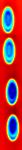
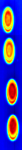
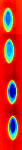
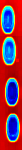
In addition to the KernelSize that can be modified, there is also the StructuringElement parameter, which indicates which shape the kernel should have when looking at neighboring pixels. A simple Square kernel will be a square of the given size; a Disk will be a circle of that radius (only pixels that have a distance of at most exactly the radius will be considered part of the kernel); a Cross kernel will only include pixels along the x and y axis starting from the current point. The following images show the shapes of the kernels for 2D (in the 5x5 case):
Square |
Cross |
Disc |
|
|
|
|
Example Data
The following table shows the effect of the kernel filter at default parameters when applied to grayscale data:
Input |
GradientModulus |
Laplace |
Gaussian |
LoG |
BoxBlur |
Dilation |
Erosion |
|
|
|
|
|
|
|
|
|
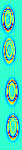

(The Dilation and Erosion appear to have the inverse effect as desribed, but this is because this example data has a highly reflective background (close to 1), while the objects themselves reflect less light, so the effect is opposite to the effect that one might naively expect from these kernels.)
When applied to mask data, the following table shows the output of the filter when using default parameters:
Input |
Dilation |
Erosion |
|
|
|
|

Sequenced Operations (Line Cameras)
The Kernel Operation filter also works with line cameras (or in the case of hyperspectral cameras, Push Brooms) that pass in data line by line. However, since the filter needs to look at lines that will only come after the current line, this is solved by introducing a delay. For exmaple, if the kernel size is 3, when the first line is being processed, this filter will output nothing. Once the second line is being processed, the filter is able to output the result for the first line (because it can now look at the second line). The output of the filter hence has a delay of 1 line.
The processing framework will automatically take care of delays when the filter is then connected to other filters. For example, if one constructs a graph with the following node sequence:
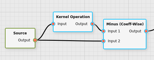
Then the framework will ensure that the coefficient-wise subtraction filter will see the data belonging to the same pixels while subtracting them. This means that filter will have a delay of 1 as well, as a consequence of the delay that was introduced by the Kernel Operation filter.
Hence the user need not keep track of the delay themselves, as the processing framework will take care of that. However, if the user wants to perform inline processing with fluxEngine, they must be able to handle the fact that such a delay can be introduced. (The delay of any output can be queried in fluxEngine.)
The size of the delay is given by half the kernel size, rounded down.
For example, a kernel of size 7 will introduce a delay of
 . The implicit size of the
GradientModulus kernel is 3 (hence a delay of 1 in that case).
. The implicit size of the
GradientModulus kernel is 3 (hence a delay of 1 in that case).